Cubic smoothing splines embody a curve fitting technique which blends the ideas of cubic splines and curvature minimization to create an effective data modeling tool for noisy data. Traditional interpolating cubic splines represent the tabulated data as a piece-wise continuous curve which passes through each value in the data table. The curve spanning each data interval is represented by a cubic polynomial, with the requirement that the endpoints of adjacent cubic polynomials match in location and in their first and second derivatives. If we need to fit a spline to some non-uniformly sampled noisy data, the results can be rather unsatisfying because every data point is visited by the spline (see chart below).
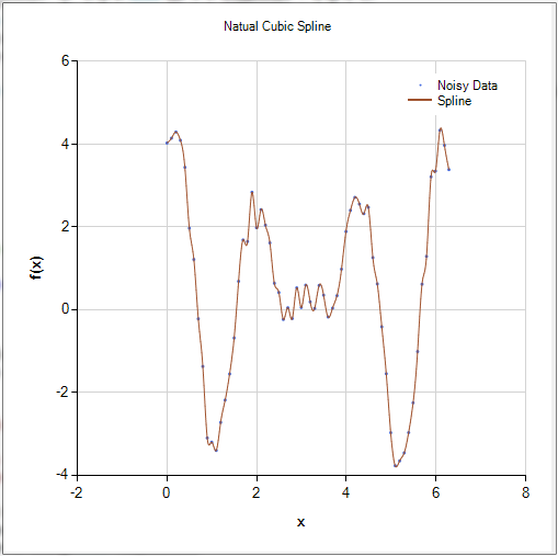
If a smoothed cubic spline is fitted to the same noisy dataset, the general sense of the data is captured without the spline mimicking the noise.

Understanding Smoothing Cubic Splines
Both cubic splines and cubic smoothing splines are constrained to have contiguous first and second derivatives, however only (interpolating) cubic splines are required to pass though all data points. Freed of these N data-point constraints, new additional constraints are now needed to have a fully determined solution. In the case of cubic smoothing splines we have the following two functional constraints: one which minimizes the squared error between the data and spline, and a second which minimizes the curvature.
To minimize the squared error we minimize the following function, where the yi‘s are the data’s ordinates, and the g(x)‘s are cubic polynomials.
To minimize the curvature we minimize:
Since we are not concerned with the convexity or concavity of the curvature, only the amount of curvature, we square the curvature eliminating the sign.
For most data sets, these two constraint functions act in opposition to one another. The first constraint pushes the spline as close as possible to the data points while the second attempts to keep the spline as free of curvature as possible. In the final formulation, these two countervailing constraints are joining by a weighting parameter, p, which balances these two opposing constraints and results in a smoothing cubic spline.
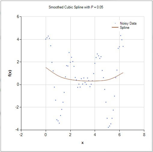
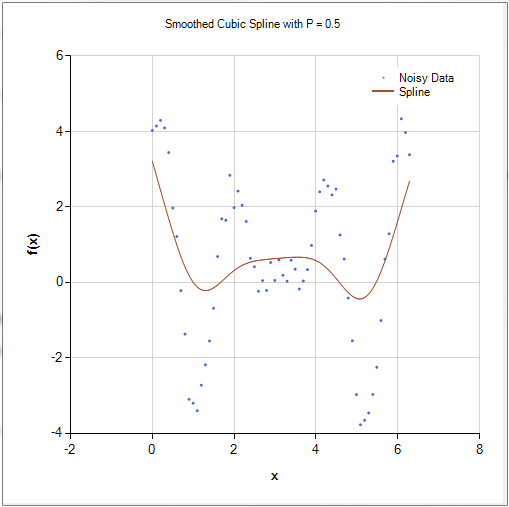
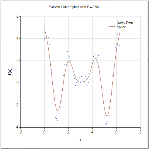
The two degenerate cases are worth pondering. If p = 1 the curvature constraint is nullified and the smoothing cubic spline then passes through all data points resulting in an interpolation spline. In other words, with p = 1 we have reverted back to a natural cubic spline solution. If p = 0 only the curvature of the spline is minimized. Therefore we are minimizing the mean squared error over linear functions resulting in a linear (straight-line) least squares fit. A few smoothing cubic splines are shown below demonstrating the effect of various choices of p.
Smoothing Cubic Splines C# code example.
The NMath library currently supports two spline classes for natural and clamped splines. The class SmoothCubicSpline is not currently released but will be available in the spring 2014 release of NMath 6.0. If you have a need for this class before our next release, please contact us.
|
NMath Class Name
|
Description
|
|---|---|
|
Natural cubic spline
|
|
|
Clamped cubic spline
|
|
|
Smoothing cubic spline
|
The following example code creates a noisy sinusoid signal then generates a smoothing cubic spline fit and finally charts the results.
// Build a noisy signal to fit with the smooth cubic spline.
var numPoints = 64;
x = new DoubleVector( numPoints, 0, 2.0 * Math.PI / ( numPoints - 1.0 ) );
yNoisy = new DoubleVector( numPoints );
RandGenUniform rng = new RandGenUniform( 0x162 );
for ( int i = 0; i < x.Length; i++ )
{
yNoisy[i] = ( 2.3 * Math.Cos( 3.0 * x[i] ) +
1.2 * Math.Sin( 4.5 * x[i] ) +
Math.Cos( 1.92 * x[i] ) ) + rng.Next();
}
// Compute the cubic smoothing spline.
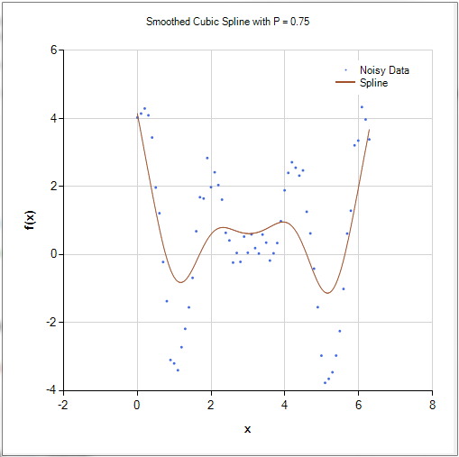
double p = 0.75;
SmoothCubicSpline spline = new SmoothCubicSpline( x, yNoisy, p );
// Chart the noisy signal and smoothing spline.
var numInterpolatedValues = 512;
var chart = NMathChart.ToChart( spline, numInterpolatedValues );
chart.Titles.Add( String.Format( "Smoothed Cubic Spline with P = {0}", p.ToString() ) );
chart.Series[0].Name = "Noisy Data";
chart.Series[1].Name = "Spline";
NMathChart.Show( chart );
The above code was used to generate the following four charts which compare cubic spline fits of the same dataset with different weighting factors. The four weighting factors used were p = 0.05, 0.5, 0.75, 0.98.
 |
 |
 |
 |
It’s worth noting that if you need to filter uniformly sampled data Savitzky-Golay filters work similarly to a cubic smoothing spline by fitting piecewise continuous polynomials to the data. To more learn about Savitzky-Golay filtering have a look at our blog article.
-Happy Computing,
Paul Shirkey
References
P. Craven and G. Wahba, “Smoothing Noisy Data with Spline Functions”, Numerische Mathematik, vol. 31, pp. 377-403, 1979.