Principal Components Regression: Recap of Part 2
Recall that the least squares solution 

(1)

And that problems occurred finding 
(2)
was close to being singular. The Principal Components Regression approach to addressing the problem is to replace 
(3)
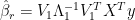
where 
are the corresponding eigenvectors of

[eds: This blog article is final entry of a three part series on principal component regression. The first article in this series, “Principal Component Regression: Part 1 – The Magic of the SVD” is here. And the second, “Principal Components Regression: Part 2 – The Problem With Linear Regression” is here.]
Review: Eigenvalues and Singular Values
In order to develop the algorithm, I want to go back to the Singular Value Decomposition (SVD) of a matrix and its relationship to the eigenvalue decomposition. Recall that the SVD of a matrix X is given by
(4)

Where U is the matrix of left singular vectors, V is the matrix of right singular vectors, and Σ is a diagonal matrix with positive entries equal to the singular values. The eigenvalue decomposition of
(5)
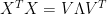
Where the eigenvalues of X are the diagonal entries of the diagonal matrix 
Recall further that if the matrix X has rank r then X can be written as
(6)

Where 


Principal Components
The subject here is Principal Components Regression (PCR), but we have yet to mention principal components. All we have talked about are eigenvalues, eigenvectors, singular values, and singular vectors. We’ve seen how singular stuff and eigen stuff are related, but what are principal components?
Principal component analysis applies when one considers statistical properties of data. In linear regression each column of our matrix X represents a variable and each row is a set of observed value for these variables. The variables being observed are random variables and as such have means and variances. If we center the matrix X by subtracting from each column of X its corresponding mean, then we’ve normalized the random variables being observed so that they have zero mean. Once the matrix X is centered in this way, the matrix
In the SVD given by equation (4), define the matrix T by
(7)

The matrix T is called the scores for X. Note that T is orthogonal, but not necessarily orthonormal. Substituting this into the SVD for X yields
(8)

Using the fact that V is orthogonal we can also write
(9)

We call the matrix V the loadings. The goal of our algorithm is to obtain the representation given by equation (8) for X, retaining all the most significant principal components (or eigenvalues, or singular values – depending on where your heads at at the time).
Computing the Solution
Using equation (3) to compute the solution to our problem involves forming the matrix
The NIPALS Algorithm
We will be using an algorithm known as NIPALS (Nonlinear Iterative PArtial Least Squares). The NIPALS algorithm for the matrix X in our least squares problem and r, the number of retained principal components, proceeds as follows:
Initialize 

- Choose
as any column of
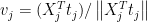
- Let
- Let
- If
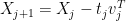
- Let
- If
stop. Otherwise increment j and return to step 1.


Properties of the NIPALS Algorithm
Let us see how the NIPALS algorithm produces principal components for us.
Let 
(10)

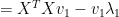
Setting 
(11)
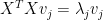
This equation is satisfied upon completion of the loop 2-4. This shows that 


(12)


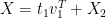
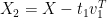
After one iteration of the NIPALS algorithm we end up at step 5 with
(13)
Note that 
are orthogonal:
(14)


Furthermore, since 

, whose columns are the vectors
,
whose columns are the
,
(15)

If r is equal to the rank of X then, using the information obtained from equations (12) and (14), it follows that (15) yields the matrix decomposition (8). The idea behind Principal Components Regression is that after choosing an appropriate r the important features of X have been captured in
(16) 
The least squares solution then gives
(17)

Note that since 
(18)

From (18) we see that the PCR estimation 
(19) 
Steve