SIGA, a public biotechnology company, recently hired CenterSpace consultants to refine their logistic modeling capabilities. Modeling a dose-response system with a logistic curve is one important special case of the more general non-linear curve fitting problem. If you are familiar with linear regression and related statistics, the non-linear case closely parallels the linear case making the jump to non-linear curve fitting easier.
SIGA is a world leader in designing and developing novel countermeasures to prevent and treat serious infectious diseases, with an emphasis on biological warfare defense. |
In a previous blog post, Ken outlined the techniques for using NMath to compute various common linear trend lines and non-linear trend lines linearizable via a simple variable substitution. This post extends that curve fitting article to the non-linear case.
Non-linear Curving Fitting – The Logistic
The logistic model is a fundamental non-linear model for many systems, and is widely used in the life sciences, medicine, and environmental toxicology.
 |
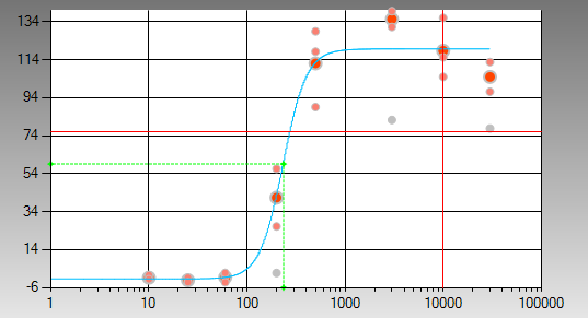
This image shows a fit of a 4-parameter logistic model to the measured inhibitory response of an infectious agent to a treatment at various drug dose levels – this is a classic dose-response curve. The 4-parameter model was used here because the underlying physical process is expected to be symmetric, and is defined as:
| a – response at x = 0 | b – slope factor | c – mid-range (50%) concentration | d – response as x -> infinity |
The 5-parameter logistic adds an additional asymmetry parameter that allow the leading and trailing tails to have different curvatures. It is defined as:
| a – response at x = 0 | b – slope factor | c – mid-range (50%) concentration | d – response as x -> infinity | g – asymmetry factor |
Using NMath the following C# code fits the four-parameter logistic to the given data. By extending the initial conditions vector by one element, and changing the model function delegate we could use the same code to fit the FiveParameterLogistic function.
using CenterSpace.NMath.Core;
using CenterSpace.NMath.Analysis;

 public void NonlinearFitExampleCode()
 {
    // Make some synthetic data
    DoubleVector xValues = new DoubleVector("30000 10000 3000 500 200 60  25 10");
    DoubleVector yValues = new DoubleVector("112.8 115 131 118 26 1.7 -0.8 -1.4");

    // This is the function delegate that the curve fitting
    // class will use - any delegate can be used.
    NMathFunctions.GeneralizedDoubleUnaryFunction f
      = AnalysisFunctions.FourParameterLogistic;

    // The starting point in the function parameter space.
    DoubleVector start = new DoubleVector("0.1 0.1 0.1 0.1");

    // Construct a curve fitting object for our function, then perform the fit.
    OneVariableFunctionFitter fitter
      = new OneVariableFunctionFitter(f);
    DoubleVector solution = fitter.Fit(xValues, yValues, start);

    // Display solution
    Console.WriteLine("4 Parameter Logistic Model Parameters: {0}", solution.ToString("0.####"));
}
The model parameters are returned in a vector, in the order defined above [a, b, c, d].
4 Parameter Logistic Model Parameters:
  [ -0.1755 6.0556 246.8343 119.6108 ]
The fitting class OneVariableFunctionFitter is based on the Trust Region algorithm which is an extension of the Levenberg-Marquardt minimization algorithm. As used in the example above, the partial derivatives with respect to the parameters are numerically estimated. In our experience numerically estimating the partials works very well. However, for improved precision and performance it is also possible to explicitly specify delegates for the partials, using the property:
NMathFunctions.GeneralizedDoubleUnaryFunction[] PartialDeriviates
If the curvature of the function surface is low, as is typically the case for the logistic model, and the local linearized estimate closely approximates the function surface during the minimization process, the partial derivatives are not even evaluated for performance reasons.
Bounded Parameters
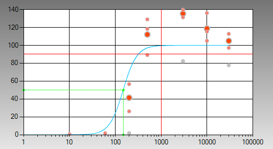
Because the OneVariableFunctionFitter is based on the Trust Region algorithm, it is possible to place bounds on the parameters. This is a very powerful feature, which is frequently employed when modeling a dose-response curve with a logistic. There’s an old debate between the chemists and biologists regarding the dose-response curve on whether the curve should be relative or absolute. In the image above, a relative dose-response curve is shown, as there were no bounds placed on the four parameters. However, we can create an absolute dose-response curve by adding the constraints 100 >= a >= 0 and 0 <= d <= 100 and re-fitting the curve. This will enforce all predicted responses to be between 0% and 100%.
Here is a C# code example on how to do this with NMath.
using CenterSpace.NMath.Core;
using CenterSpace.NMath.Analysis;

 public void BoundedNonlinearFitExampleCode()
 {

  // Make some synthetic data
  DoubleVector xValues = new DoubleVector("30000 10000 3000 500 200 60  25 10");
  DoubleVector yValues = new DoubleVector("112.8 115 131 118 26 1.7 -0.8 -1.4");

  // The starting point in the function parameter space.
  DoubleVector start = new DoubleVector("0.1 0.1 0.1 100.0");

  // 4-parameter bounds in the order of a, b, c, & d
  DoubleVector lowerBounds = new DoubleVector("0.0 0.0 0.0 0.0");
  DoubleVector upperBounds = new DoubleVector("100.0 100000.0 100000.0 100.0");

  // Convert the 4-parameter logistic to a Func<>
  Func<Double[], Double, Double> fitFunction =
    new Func<double[], double, double>((double[] soln, Double x) => AnalysisFunctions.FourParameterLogisticFunction(new   DoubleVector(soln), x));

  // This class is not included with the current release.
  FunctionFitterWithBounds fitter =
    new FunctionFitterWithBounds(fitFunction, lowerBounds, upperBounds);

  //Now define and fit the data as shown above.
  DoubleVector solution = fitter.Fit(xValues, yValues, start);

  // Display solution
   Console.WriteLine("4 Parameter Logistic Model Parameters: {0}", solution.ToString("0.####"));
}
The bounded model parameters returned, in the order defined above [a, b, c, d] are:
4 Parameter Logistic Model Parameters: [ 0 0.1652 0.787 100 ]
Note that the first and last parameters are now within the specified bounds.
The class FunctionFitterWithBounds is unreleased (and won’t be in this form) but you can download it and use it if you have the latest release of NMath installed. The non-linear curving fitting NMath API will be extended and refined in our next NMath release, and bounded non-linear curve fitting will be more clearly accessible.
Update: Bounded non-linear curve fitting is now included in NMath.
Goodness-Of-Fit Model Statistics
After we are done fitting our model, the fit may look good, but really how good is the fit? To better understand the goodness-of-fit of our model, we need to analyze the residuals of the fit and related statistics. The next release of NMath Stats (expected in June) will offer a new class GoodnessOfFit that will provide a complete set of statistical measures that can be used to assess the goodness-of-fit for a non-linear model, including the F-Statistic, t-Statistic, and parameter confidence intervals. Please contact us if you are interested in obtaining an advanced copy of this class.
Happy Computing,
Paul
Resources
- The five-parameter logistic: A characterization and comparison with the four-parameter logistic, Paul G. Gotschalk, John R. Dunn, Analytical Biochemistry 343 (2005) pp 54-65.
- Principles of Curve Fitting for Multiplex Sandwich Immunoassays, D. Davis, A. Zhang, C. Etienne, I. Huang, & M. Malit, tech note 2861.
- A brief technical introduction to Trust Region methods, by Mark S. Gockenbach


One thought on “Non-linear Curve Fitting”