In this continuing series, we explore the NMath Stats functions for performing cluster analysis in .NET. (For previous posts, see here.) The sample data set we’re using classifies 89 single malt scotch whiskies on a five-point scale (0-4) for 12 flavor characteristics. To visualize the data set and clusterings, we make use of the free Microsoft Chart Controls for .NET, which provide a basic set of charts.
In this post, we’ll cluster the scotches based on “similarity” in the original 12-dimensional flavor space using k-means clustering. The k-means clustering method assigns data points into k groups such that the sum of squares from points to the computed cluster centers is minimized. In NMath Stats, class KMeansClustering performs k-means clustering.
The algorithm used is that of Hartigan and Wong (1979):
- For each point, move it to another cluster if that would lower the sum of squares from points to the computed cluster centers.
- If a point is moved, immediately update the cluster centers of the two affected clusters.
- Repeat until no points are moved, or the specified maximum number of iterations is reached.
A KMeansClustering instance is constructed from a matrix or a dataframe containing numeric data. Each row in the data set represents an object to be clustered. The Cluster() method clusters the data into the specified number of clusters. The method accepts either k, the number of clusters, or a matrix of initial cluster centers:
- If k is given, a set of distinct rows in the data matrix are chosen as the initial centers using the algorithm specified by a KMeanClustering.Start enumerated value. By default, rows are chosen at random.
- If a matrix of initial cluster centers is given, k is inferred from the number of rows.
For example, this C# code clusters the scotch data (loaded into a dataframe in Part I) into four clusters:
KMeansClustering km = new KMeansClustering(df);
int k = 4;
km.Cluster(k, KMeansClustering.Start.QuickCluster);
K-means clustering requires a set of starting cluster centers to initiate the iterative algorithm. By default, rows are chosen at random from the given data. Here we employ the QuickCluster algorithm, similar to the SPSS QuickCluster function, for choosing the starting centers. (The QuickCluster algorithm proceeeds as follows: If the distance between row r and its closest center is greater than the distance between the two closest centers (m, n), then r replaces m or n, whichever is closest to r. Otherwise, if the distance between row r and its closest center (q) is greater than the distance between q and its closest center, then row r replaces q.)
The Clusters property returns a ClusterSet object, which represents a collection of objects assigned to a finite number of clusters. The following C# code prints out the members of each cluster:
ClusterSet cs = km.Clusters;
for (int i = 0; i < cs.NumberOfClusters; i++)
{
     Console.WriteLine("Cluster {0} contains:", i);
     int[] members = cs.Cluster(i);
     for (int j = 0; j < members.Length; j++)
     {
          Console.Write("{0} ", df.RowKeys[members[j]]);
     }
     Console.WriteLine("\n");
}
The output looks like this:
Cluster 0 contains:
Aberfeldy Aberlour Ardmore Auchroisk Balmenach Belvenie
BenNevis Benriach Benrinnes Benromach BlairAthol Craigallechie
Dailuaine Dalmore Deanston Edradour GlenKeith GlenOrd
Glendronach Glendullan Glenfarclas Glenlivet Glenrothes
Glenturret Knochando Linkwood Longmorn Macallan Mortlach
OldFettercairn RoyalLochnagar Scapa Strathisla

Cluster 1 contains:
Ardbeg Caol Ila Clynelish Lagavulin Laphroig Talisker

Cluster 2 contains:
AnCnoc Auchentoshan Aultmore Bladnoch Bunnahabhain
Cardhu Craigganmore Dalwhinnie Dufftown GlenElgin GlenGrant
GlenMoray GlenSpey Glenallachie Glenfiddich Glengoyne
Glenkinchie Glenlossie Inchgower Loch Lomond Mannochmore
Miltonduff Speyburn Speyside Strathmill Tamdhu Tamnavulin
Tobermory Tomintoul Tomore Tullibardine

Cluster 3 contains:
ArranIsleOf Balblair Bowmore Bruichladdich GlenDeveronMacduff
GlenGarioch GlenScotia Glenmorangie Highland Park Isle of Jura
Oban OldPulteney RoyalBrackla Springbank Teaninich Tomatin
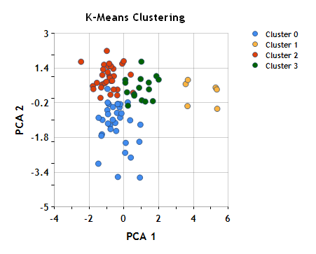
To help visualize these clusters, we can once again plot the scotches in the plane formed by the first two principal components (see Part I), which collectively account for ~50% of the variance, coloring the points based on cluster assignment.

Remember that although we’ve used dimension reduction (principal component analysis, in this case) to visualize the clustering, the clustering itself was performed based on similarity in the original 12-dimensional flavor space, not based on distance in this plane. Nonetheless, the clusters look pretty reasonable.
K-means clustering is very efficient for large data sets, but does require you to know the number of clusters, k, in advance. Also, you have no control of the similarity metric used to cluster the objects (within-cluster sum of squares). In the next post in this series, we’ll look at hierarchical cluster analysis, which constructs the entire hierarchical cluster tree, and allows you to specify the distance and linkage functions to use.
Ken
References
Hartigan, J.A. and Wong, M.A. (1979). A k-means clustering algorithm. Algorithm AS136, Appl. Stat. 28, pp. 100–108.

2 thoughts on “Clustering Analysis, Part II: K-Means Clustering”