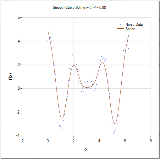
Savitzky-Golay smoothing effectively removes local signal noise while preserving the shape of the signal. Commonly, it’s used as a preprocessing step with experimental data, especially spectrometry data, because of it’s effectiveness at removing random variation while minimally degrading the signal’s information content. Savitzky-Golay boils down to a fast (multi-core scaling) correlation operation, and therefore can be used in a real-time environment or on large data sets. If higher order information is needed from the signal, Savitzky-Golay can also provide high quality smoothed derivatives of a noisy signal.
Algorithm
Savitzky-Golay locally smooths a signal by fitting a polynomial, in a least squares sense, to a sliding window of data. The degree of the polynomial and the length of the sliding window are the filter’s two tuning parameters. If n is the degree of the polynomial that we are fitting, and k is the width of the sliding window, then

is needed for smoothing behavior (we must avoid an over-determined system). Typically
n is 3 or 4, and
k depends on the size in samples of the noisy features to be suppressed in your dataset.
For the case of n=0 the Savitzy-Golay filter degenerates to a moving average filter – which is good for removing white noise, but is poor for preserving peak shape (higher order moments). For n=1, the filter does a linear least-squares fit of the windowed data to a line. If n=k-1, the polynomial exactly fits data point in the window, and so no filtering takes place.
Once the polynomial is fit, then (typically) the center datapoint in this window is replaced by value of the polynomial at that location. The window then slides to the right one sample, and the process is repeated.
Savizky-Golay delivers the unexpected surprise that the polynomial fitting coefficients are constant for a given n and k. This means that once we fix n and k for our filter, the Savizky-Golay polynomial fitting coefficients are computed once during setup, and then used across the entire data set. This is why Savizky-Golay is a high performance correlation filter.
Comparison Example
The following three images show some real experimental data and a comparison of two filtering algorithms. The first image shows the raw data, the second image shows the effect of an averaging filter, and the last image demonstrates a Savitzky-Golay smoothing filter of length five.

Raw Data

Averaging Filter, Length 5

Savitzky-Golay Smoothing, Length 5
The averaging filter introduces a large error into the location of the orange peak, whereas Savitzky-Golay removes the noise while maintaining the peak location. Computationally, they require identical effort.
NMath Stats Code Example
The Savitzky-Golay smoothing filter is implemented in the NMath-Stats package as a generalized correlation filter. Any filter coefficients can be used with this moving window filter, Savitzky-Golay are just one possibility. The moving window filter also does not require the filtering to take place in the center of the sliding window; so when specifying the window, two parameters are required: number to the left, and number to the right, of the filtered data point.
Here are the key software components.
- MovingWindowFilter.
SavitzkyGolayCoefficients(nLeft, nRight, PolyDeg)
- MovingWindowFilter(nLeft, nRight, Coefficients[])
- MovingWindowFilter.Filter(data, boundary options)
The first is a static function for generating the Savizky-Golay coefficients, the second is the filtering class that takes the generated coefficients in the constructor. The third is the method that actually does the filtering by running a cross-correlation between the data the the saved coefficients.
Below is a complete code example to copy and experiment with. Only three lines of code are needed to build the filter and do the filtering. The remaining code is for displaying results and building a synthetic noisy signal.
int nLeft = 2;
int nRight = 2;
int n = 3;
// Generate the coefficients.
DoubleVector c =
MovingWindowFilter.SavitzkyGolayCoefficients( nLeft, nRight, n );
// Build the filter of width: nLeft + nRight + 1
MovingWindowFilter filter =
new MovingWindowFilter( nLeft, nRight, c );
Console.WriteLine( "Filter coeffs = " + filter.Coefficients );
// Generate a signal
DoubleVector x = new DoubleVector( 100, -5, .1 );
DoubleVector y = new DoubleVector( x.Length );
for ( int i = 0; i < x.Length; i++ )
{
double a = x[i];
y[i] = 0.03*Math.Pow(a, 3) + 0.2*Math.Pow(a, 2) -.22*a + 0.5;
}
Console.WriteLine( "Smoothed signal = " + y );
RandGenUniform rng = new RandGenUniform(-1, 1, 0x124 );
for ( int i = 0; i < y.Length; i++ )
{
y[i] += rng.NextDouble();
}
Console.WriteLine( "x = " + x );
Console.WriteLine( "Noisy signal = " + y );
// Do the filtering.
DoubleVector z =
filter.Filter(y, MovingWindowFilter.BoundaryOption.PadWithZeros);
Console.WriteLine( "Signal filtered = " + z );
-Paul
Addendum – Savitzky-Golay Coefficients
If you want to quickly try out Savitzky-Golay smoothing without computing the coefficients, or just compare coefficients, here are some coefficients for a sliding window of length five. They also provide some insight into the relationship between the coefficients and the behavior of the filter.
Filter length = 5, nLeft = 2, nRight = 2.
Polynomial of order 0,
[ 0.2 0.2 0.2 0.2 0.2 ] (averaging filter)
Polynomial of order 1,
[ 0.2 0.2 0.2 0.2 0.2 ]
Polynomial of order 2,
[ -0.0857142 0.3428571 0.4857142 0.3428571 -0.0857142 ]
Polynomial of order 3,
[ -0.0857142 0.3428571 0.4857142 0.3428571 -0.0857142 ]
Polynomial of order 4 and higher,
[ 0 0 1 0 0 ] (as expected, no filtering here!)
Another Smoothing Example on Real Data
This is another example of Savitzky-Golay smoothing on some experimental data. If more smoothing was desired, a longer filtering window could have been used.

Savitzky-Golay Smoothing, Length = 5.