Chromatographic and spectographic data analysis is a common application of the NMath class library and usually involves some or all of the following computing activities:
- Noise removal
- Baseline adjustment
- Peak finding
- Peak modeling
- Peak statistical analysis
In this blog article we will discuss each of these activities and provide some NMath C# code on how they may be accomplished. This is big subject but the goal here is to get you started solving your spectographic data analysis problems, perhaps introduce you to a new technique, and finally to provide some helpful code snippets that can be expanded upon.
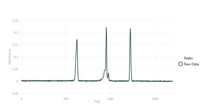
Throughout this article we will be using the following electrophoretic data set below in our code examples. This data set contains four obvious peaks and one partially convolved peak infilled with underlying white noise.

Noise Removal
Chromatographic, spectographic, fMRI or EEG data, and many other types of time series are non-stationary. This non-stationarity means that Fourier based filtering methods are ill suited to removing noise from these signals. Fortunately we can effectively apply wavelet analysis, which does not depend on signal periodicity, to suppress the signal noise without altering the signal’s phase or magnitude. Briefly, the discrete wavelet transform (DWT) can be used to recursively decompose the signal successively into details and approximations components. From a filtering perspective the signal details contain the higher frequency parts and the approximations contain the lower frequency components. As you’d expect the inverse DWT can elegantly reconstruct the original signal but, to meet our noise removal goals, the higher frequency noisy parts of the signal can be suppressed during the signal reconstruction and be effectively removed. This technique is called wavelet shrinkage and is described in more detail in an earlier blog article with references.

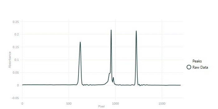
These results can be refined, but this starting point is seen to have successfully removed the noise but not altered the position or general shape of the peaks. Choosing the right wavelet for wavelet shrinkage is done empirically with a representative data set at hand.
public DoubleVector SuppressNoise( DoubleVector DataSet  )
{
  var wavelet = new DoubleWavelet( Wavelet.Wavelets.D4 );
  var dwt = new DoubleDWT( DataSet.ToArray(), wavelet );
  dwt.Decompose( 5 );
  double lambdaU = dwt.ComputeThreshold( FloatDWT.ThresholdMethod.Sure, 1 );

  dwt.ThresholdAllLevels( FloatDWT.ThresholdPolicy.Soft, new double[] { lambdaU, lambdaU, lambdaU, lambdaU, lambdaU } );

  double[] reconstructedData = dwt.Reconstruct();
  var filteredData= new DoubleVector( reconstructedData );
  return filteredData;
}
With our example data set a Daubechies 4 wavelet worked well for noise removal. Note that the same threshold was applied to all DWT decomposition levels; Improved white noise suppression can be realized by adopting other thresholding strategies.
Baseline Adjustment
Dozens of methods have been developed for modeling and removing a baseline from various types of spectra data. The R package baseline has collected together a range of these techniques and can serve as a good starting point for exploration. The techniques variously use regression, iterative erosion and dilation, spectral filtering, convex hulls, or partitioning and create baseline models of lines, polynomials, or more complex curves that can then be subtracted from the raw data. (Another R package, MALDIquant, contains several more useful baseline removal techniques.) Due to the wide variety of baseline removal techniques and the lack of standards across datasets, NMath does not natively offer any baseline removal algorithms.
Example baseline modeling
The C# example baseline modeling code below uses z-scores and iterative peak suppression to create a polynomial model of the baseline. Peaks that extend beyond 1.5 z-scores are iteratively cut down by a quarter and then a polynomial is fitted to this modified data set. Once the baseline polynomial fits well and stops improving upon iterative suppression the model is returned.
private PolynomialLeastSquares findBaseLine( DoubleVector x, DoubleVector y, int PolynomialDegree )
 {
   var lsFit = new PolynomialLeastSquares( PolynomialDegree, x, y );
   var previousRSoS = 1.0;

   while ( lsFit.LeastSquaresSolution.ResidualSumOfSquares > 0.1 && Math.Abs( previousRSoS - lsFit.LeastSquaresSolution.ResidualSumOfSquares ) > 0.00001 )
   {
     // compute the Z-scores of the residues and erode data beyond 1.5 stds.
     var residues = lsFit.LeastSquaresSolution.Residuals;
     var Zscores = ( residues - NMathFunctions.Mean( residues ) ) / Math.Sqrt( NMathFunctions.Variance( residues ) );
     previousRSoS = lsFit.LeastSquaresSolution.ResidualSumOfSquares;

     y[0] = Zscores[0] > 1.5 ? 0 : y[0];
     for ( int i = 1; i < this.Length; i++ )
     {
       if ( Zscores[i] > 1.5 )
       {
         y[i] = y[i-1] / 4.0;
       }
     }
     lsFit = new PolynomialLeastSquares( PolynomialDegree, x, y );
    }
    return lsFit;
 }
This algorithm has proven reliable for estimating both 1 and 2 degree polynomial baselines with electrophoretic data sets. It is not designed to model the wandering baselines sometimes found in mass spec data. The SNIP [2] method or Asymmetric Least Squares Smoothing [1] would be better suited for those data sets.
Peak Finding
Locating peaks in a data set usually involves, at some level, finding the zero crossings of the first derivative of the signal. However, directly differentiating a signal amplifies noise and so more sophisticated indirect methods are usually employed. Savitzky-Golay polynomials are commonly used to provide high quality smoothed derivatives of a noisy signal and are widely employed with chromatographic and other data sets (See this blog article for more details).

// Code snippet for locating peaks.
var sgFilter = new SavitzkyGolayFilter( 4, 4, 2 );
DoubleVector filteredData = sgFilter.Filter( DataSet );
var rbPeakFinder = new PeakFinderRuleBased( filteredData );
rbPeakFinder.AddRule( PeakFinderRuleBased.Rules.MinHeight, 0.005 );
List<int> pkIndicies = rbPeakFinder.LocatePeakIndices();
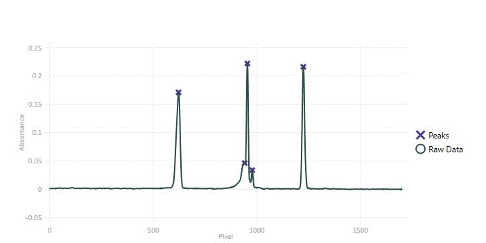
Without thresholding many small noisy undulations are returned as peaks. Thresholding with this data set works well in separating the data peaks from the noise, however sometimes peak modeling is necessary for separating data peaks from noise when they are both present at similar scales.
Peak Modeling and Statistics
In addition to separating out false peaks, peaks are also modeled to compute various peak statistical measures such as FWHM, CV, area, or standard deviation. The Gaussian is an excellent place to start for peak modeling and for many applications this model is sufficient. However there are many other peak models including: Lorenzian, Voigt, [3] CSR, and variations on exponentially modified Gaussians (EMG’s). Many combinations, convolutions, and refinements of these models are gathered together and presented in a useful paper by DeMarko & Bombi, 2001. Their paper focused on chromatographic peaks but the models surveyed therein have wide application.
/// <summary>
/// Gaussian Func<> for trust region fitter.
/// p[0] = mean, p[1] = sigma, p[2] = baseline offset
/// </summary>
private static Func<DoubleVector, double, double> Gaussian = delegate ( DoubleVector p, double x )
{
   double a = ( 1.0 / ( p[1] * Math.Sqrt( 2.0 * Math.PI ) ) );
   return a * Math.Exp( -1 * Math.Pow( x - p[0], 2 ) / ( 2 * p[1] * p[1] ) ) + p[2];
};
Above is a Func<> representing a Gaussian that allows for some vertical offset. The TrustRegionMinimizer in NMath is one of the most powerful and flexible methods for peak fitting. Once the start and end indices of the peaks are determined, the following code snippet fits this Gaussian model to the peak’s data.
// The DoubleVector's xValues and yValues contain the peak's data.

// Pass in the model (above) to the function fitter ctor
var modelFitter = new BoundedOneVariableFunctionFitter<TrustRegionMinimizer>( Gaussian );

// Gaussian for peak finding
var lowerBounds = new DoubleVector( new double[] { xValues[0], 1.0, -0.05 } );
var upperBounds = new DoubleVector( new double[] { xValues[xValues.Length - 1], 10.0, 0.05 } );
var initialGuess = new DoubleVector( new double[] { 0.16, 6.0, 0.001 } );

// The lower and upper bounds aren't required, but are suggested.
var soln = modelFitter.Fit( xValues, yValues, initialGuess, lowerBounds, upperBounds );

// Fit statistics
var gof = new GoodnessOfFit( modelFitter, xValues, yValues, soln );
The GoodnessOfFit class is a very useful tool for peak modeling. In one line of code one gets the f-statistics for the goodness of the fit of the model along with confidence intervals for all of the model parameters. These statistics are very useful in automating the sorting out of noisy peaks from actual data peaks and of course for determining if the model is appropriate for the data at hand.
Peak Area
Computing peak areas or peak area proportions is essential in most applications of spectographic or electrophoretic data analysis. This is this a two-liner with NMath.
// The peak starts and ends at: startIndex, endIndex.
var integrator = new DiscreteDataIntegrator();
double area =  integrator.Integrate( DataSet[ new Slice( startIndex, endIndex - startIndex + 1) ] );
The DiscreteDataIntegrator defaults to integrating with cubic spline segments. Other discrete data integration methods available are trapezoidal and parabolic.
Summary
Contact us if you need help or have questions about analyzing your team’s data sets. We can quickly help you get started solving your computing problems using NMath or go deeper and accelerate your team’s application development with consulting.
Assorted References
- Eilers, Paul & Boelens, Hans. (2005). Baseline Correction with Asymmetric Least Squares Smoothing. Unpubl. Manuscr.
- C.G. Ryan, E. Clayton, W.L. Griffin, S.H. Sie, and D.R. Cousens. 1988. SNIP, a statistics-sensitive background treatment for the quantitative analysis of pixe spectra in geoscience applications. Nuclear Instruments and Methods in Physics Research Section B: Beam Interactions with Materials and Atoms, 34(3): 396-402.
- García-Alvarez-Coque MC, Simó-Alfonso EF, Sanchis-Mallols JM, Baeza-Baeza JJ. A new mathematical function for describing electrophoretic peaks. Electrophoresis. 2005;26(11):2076-2085. doi:10.1002/elps.200410370
