Clustering Analysis, Part I: Principal Component Analysis (PCA)

Cluster analysis is the assignment of a set of objects into one or more clusters based on object similarity. NMath Stats includes a variety of techniques for performing cluster analysis, which we will explore in a series of posts.

The Data Set

The data set we’ll use was created by David Wishart (2002), who classified 89 single malt scotch whiskies on a five-point scale (0-4) for 12 flavor characteristics: Body, Sweetness, Smoky, Medicinal, Tobacco, Honey, Spicy, Winey, Nutty, Malty, Fruity, Floral. Wishart provides clusterings of the whiskies into 4, 6, and 10 clusters. Young et al. (unpublished manuscript) demonstrate a further clustering into 4 clusters using non-negative matrix factorization (NMF). Both the Young et al. paper and the original data set are available here.

Visualization

To visualize the data set and clusterings, we’ll make use of the free Microsoft Chart Controls for .NET, which provide a basic set of charts. NMath is also available as a bundle with the Syncfusion Essential Studio and Nevron Chart for .NET at a substantial discount. NMath easily interoperates with most charting packages.

Getting Started

To begin, let’s load the data set into a CenterSpace.NMath.DataFrame object:

DataFrame df =
  DataFrame.Load("ScotchWhisky01.txt", true, true, ",", true);

The parameters to the Load() method specify:

• the filename containing the data
• whether the data in the file contains column headers
• whether the data in the file contains row keys
• the column delimiter
• whether to parse the column types, or treat everything as string data.

The data set includes a leading column of row ids. Let’s replace these keys with the distillery names, then remove the distillery column from the data frame:

df.SetRowKeys(data[0]);
df.RowKeyHeader = data.ColumnHeaders[0];
df.RemoveColumn(0);

The data frame now looks like this:

Distillery     Body Sweetness Smoky Medicinal Tobacco Honey Spicy Winey Nutty Malty Fruity Floral
Aberfeldy      2 2 2 0 0 2 1 2 2 2 2 2
Aberlour       3 3 1 0 0 4 3 2 2 3 3 2
AnCnoc         1 3 2 0 0 2 0 0 2 2 3 2
Ardbeg         4 1 4 4 0 0 2 0 1 2 1 0
Ardmore        2 2 2 0 0 1 1 1 2 3 1 1
ArranIsleOf    2 3 1 1 0 1 1 1 0 1 1 2
...

There are 89 rows representing each scotch, and 12 columns representing the score on each flavor characteristic.

Principal Component Analysis

Each whisky is representing as a point in a 12-dimensional flavor space. Principal component analysis (PCA) finds a smaller set of synthetic variables that capture the maximum variance in an original data set. The first principal component accounts for as much of the variability in the data as possible, and each succeeding orthogonal component accounts for as much of the remaining variability as possible. In NMath Stats, classes DoublePCA and FloatPCA perform principal component analyses. (For more information on PCA in NMath Stats, see this page.)

For example, the following C# code constructs a PCA from the whisky data set, then prints the proportion of the variance accounted for by each principal component:

DoublePCA pca = new DoublePCA(df);
Console.WriteLine("Variance Proportions = " +
  pca.VarianceProportions);
Console.WriteLine("Cumulative Variance Proportions = " +
  pca.CumulativeVarianceProportions);

The output looks like this:

Variance Proportions =
[ 0.301109794401424 0.192178864989234 0.0956019274277357
  0.0825032185621017  0.0723086445838344 0.0599231013596576
  0.0510808855222438 0.0458706422880217  0.0349809707532734
  0.0319772808383918 0.0229738209669541 0.00949084830712784 ]

Cumulative Variance Proportions =
[ 0.301109794401424 0.493288659390658 0.588890586818394
  0.671393805380496 0.74370244996433 0.803625551323988
  0.854706436846231 0.900577079134253 0.935558049887526
  0.967535330725918 0.990509151692872 1 ]

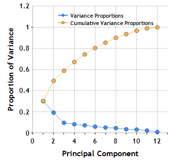
To visualize this information, we can construct a Scree plot, a simple line chart that shows the fraction of total variance in the data as explained by each principal component.

As you can see, the first two principal components account for ~50% of the variance.

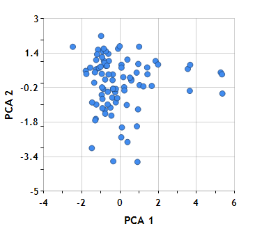
The Scores property on DoublePCA gets the score matrix. The scores are the data formed by transforming the original data into the space of the principal components. For example, here we create a view of the original 12-dimensional data by plotting the first two principal components for each scotch against each other.

The synthetic dimensions themselves are not particularly meaningful. Essentially we’ve fit a plane into the original 12-dimensional flavor space which accounts for as much of the variance as possible. This can help reveal any natural clustering. In the whisky data, however, there does not appear to be any strong natural clusters–perhaps a group of outliers at the bottom of the plot, and another group at the right. Of course, the original flavor characteristics were chosen precisely to avoid any dramatic clustering.

In future posts, we’ll apply functions in NMath Stats for k-mean clustering, hierarchical cluster analysis, and non-negative matrix factorization to explore clusterings in the data.

Ken

References

Wishart, D. (2002). Whisky Classified, Choosing Single Malts by Flavor. Pavilon, London.

Young, S.S., Fogel, P., Hawkins, D. M. (unpublished manuscript). “Clustering Scotch Whiskies using Non-Negative Matrix Factorization”. Retrieved December 15, 2009 from http://niss.org/sites/default/files/ScotchWhisky.pdf.