Distribution Fitting Demo

A customer recently asked how to fit a normal (Gaussian) distribution to a vector of experimental data. Here’s a demonstration of how to do it.

Let’s start by creating a data set: 100 values drawn from a normal distribution with known parameters (mean = 0.5, variance = 2.0).

int n = 100;
double mean = .5;
double variance = 2.0;
var data = new DoubleVector( n, new RandGenNormal( mean, variance ) );

Now, compute y values based on the empirical cumulative distribution function (CDF), which returns the probability that a random variable X will have a value less than or equal to x–that is, f(x) = P(X <= x). Here’s an easy way to do, although not necessarily the most efficient for larger data sets:

var cdfY = new DoubleVector( data.Length );
var sorted = NMathFunctions.Sort( data );
for ( int i = 0; i < data.Length; i++ )
{
  int j = 0;
  while ( j < sorted.Length && sorted[j] <= data[i] ) j++;
  cdfY[i] = j / (double)data.Length;
}

The data is sorted, then for each value x in the data, we iterate through the sorted vector looking for the first value that is greater than x.

We’ll use one of NMath’s non-linear least squares minimization routines to fit a normal distribution CDF() function to our empirical CDF. NMath provides classes for fitting generalized one variable functions to a set of points. In the space of the function parameters, beginning at a specified starting point, these classes finds a minimum (possibly local) in the sum of the squared residuals with respect to a set of data points.

A one variable function takes a single double x, and returns a double y:

y = f(x)

A generalized one variable function additionally takes a set of parameters, p, which may appear in the function expression in arbitrary ways:

y = f(p1, p2,..., pn; x)

For example, this code computes y=a*sin(b*x + c):

public double MyGeneralizedFunction( DoubleVector p, double x )
{
  return p[0] * Math.Sin( p[1] * x + p[2] );
}

In the distribution fitting example, we want to define a parameterized function delegate that returns CDF(x) for the distribution described by the given parameters (mean, variance):

Func f =
  ( DoubleVector p, double x ) =>
    new NormalDistribution( p[0], p[1] ).CDF( x );

Now that we have our data and the function we want to fit, we can apply the curve fitting routine. We’ll use a bounded function fitter, because the variance of the fitted normal distribution must be constrained to be greater than 0.

var fitter = new BoundedOneVariableFunctionFitter( f );
var start = new DoubleVector( new double[] { 0.1, 0.1 } );
var lowerBounds = new DoubleVector( new double[] { Double.MinValue, 0 } );
var upperBounds = 
   new DoubleVector( new double[] { Double.MaxValue, Double.MaxValue } );
var solution = fitter.Fit( data, cdfY, start, lowerBounds, upperBounds );
var fit = new NormalDistribution( solution[0], solution[1] );

Console.WriteLine( "Fitted distribution:\nmean={0}\nvariance={1}",
  fit.Mean, fit.Variance );

The output for one run is

Fitted distribution: 
mean=0.567334190790594
variance=2.0361207956132

which is a reasonable approximation to the original distribution (given 100 points).

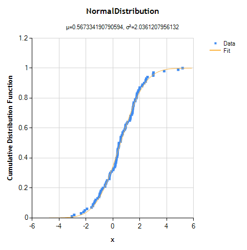
We can also visually inspect the fit by plotting the original data and the CDF() function of the fitted distribution.

ToChart( data, cdfY, SeriesChartType.Point, fit,
  NMathStatsChart.DistributionFunction.CDF );

private static void ToChart( DoubleVector x, DoubleVector y,
  SeriesChartType dataChartType, NormalDistribution dist,
  NMathStatsChart.DistributionFunction distFunction )
{
  var chart = NMathStatsChart.ToChart( dist, distFunction );
  chart.Series[0].Name = "Fit";

  var series = new Series() {
    Name = "Data",
    ChartType = dataChartType
  };
  series.Points.DataBindXY( x, y );
  chart.Series.Insert( 0, series );

  chart.Legends.Add( new Legend() );
  NMathChart.Show( chart );
}

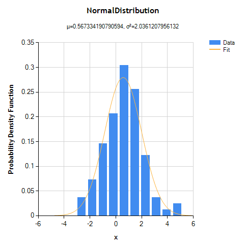
We can also look at the probability density function (PDF) of the fitted distribution, but to do so we must first construct an empirical PDF using a histogram. The x-values are the midpoints of the histogram bins, and the y-values are the histogram counts converted to probabilities, scaled to integrate to 1.

int numBins = 10;
var hist = new Histogram( numBins, data );

var pdfX = new DoubleVector( hist.NumBins );
var pdfY = new DoubleVector( hist.NumBins );
for ( int i = 0; i < hist.NumBins; i++ )
{
  // use bin midpoint for x value
  Interval bin = hist.Bins[i];
  pdfX[i] = ( bin.Min + bin.Max ) / 2;

   // convert histogram count to probability for y value
   double binWidth = bin.Max - bin.Min;
   pdfY[i] = hist.Count( i ) / ( data.Length * binWidth );
}

ToChart( pdfX, pdfY, SeriesChartType.Column, fit,
  NMathStatsChart.DistributionFunction.PDF );

You might be tempted to try to fit a distribution PDF() function directly to the histogram data, rather than using the CDF() function like we did above, but this is problematic for several reasons. The bin counts have different variability than the original data. They also have a fixed sum, so they are not independent measurements. Also, for continuous data, fitting a model based on aggregated histogram counts, rather than the original data, throws away information.

Ken

Download the source code